Reading a summer of air quality in R

A quick tour of R’s built-in airquality data with dplyr-free base R and ggplot2, plus a branded theme you can reuse.

R ships with a dataset of daily air quality readings from New York, May to September 1973. It’s small, a bit messy, and a great excuse to show off the blog’s ggplot theme.

aq <- airquality
aq$Month <- factor(month.abb[aq$Month], levels = month.abb[5:9])
knitr::kable(head(aq), caption = "First six rows")

First six rows

Ozone	Solar.R	Wind	Temp	Month	Day
41	190	7.4	67	May	1
36	118	8.0	72	May	2
12	149	12.6	74	May	3
18	313	11.5	62	May	4
NA	NA	14.3	56	May	5
28	NA	14.9	66	May	6

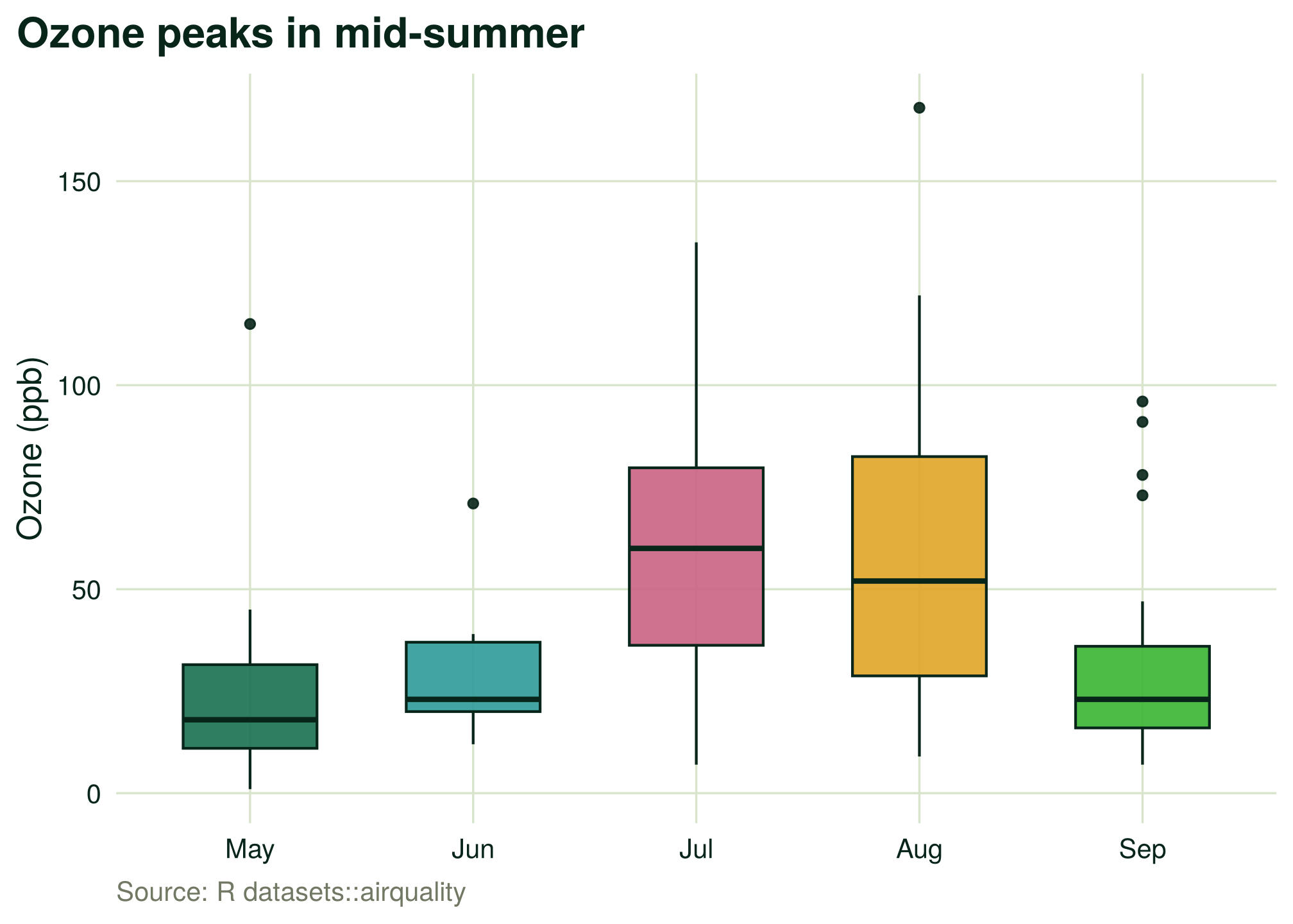
Ozone climbs through the summer

ggplot(aq, aes(Month, Ozone, fill = Month)) +
  geom_boxplot(width = 0.6, colour = fn_cols[["forest"]], alpha = 0.9, show.legend = FALSE) +
  scale_fill_StellarGrok() +
  labs(title = "Ozone peaks in mid-summer", x = NULL, y = "Ozone (ppb)",
       caption = "Source: R datasets::airquality")

Figure 1: Daily ozone by month. July and August run hottest.

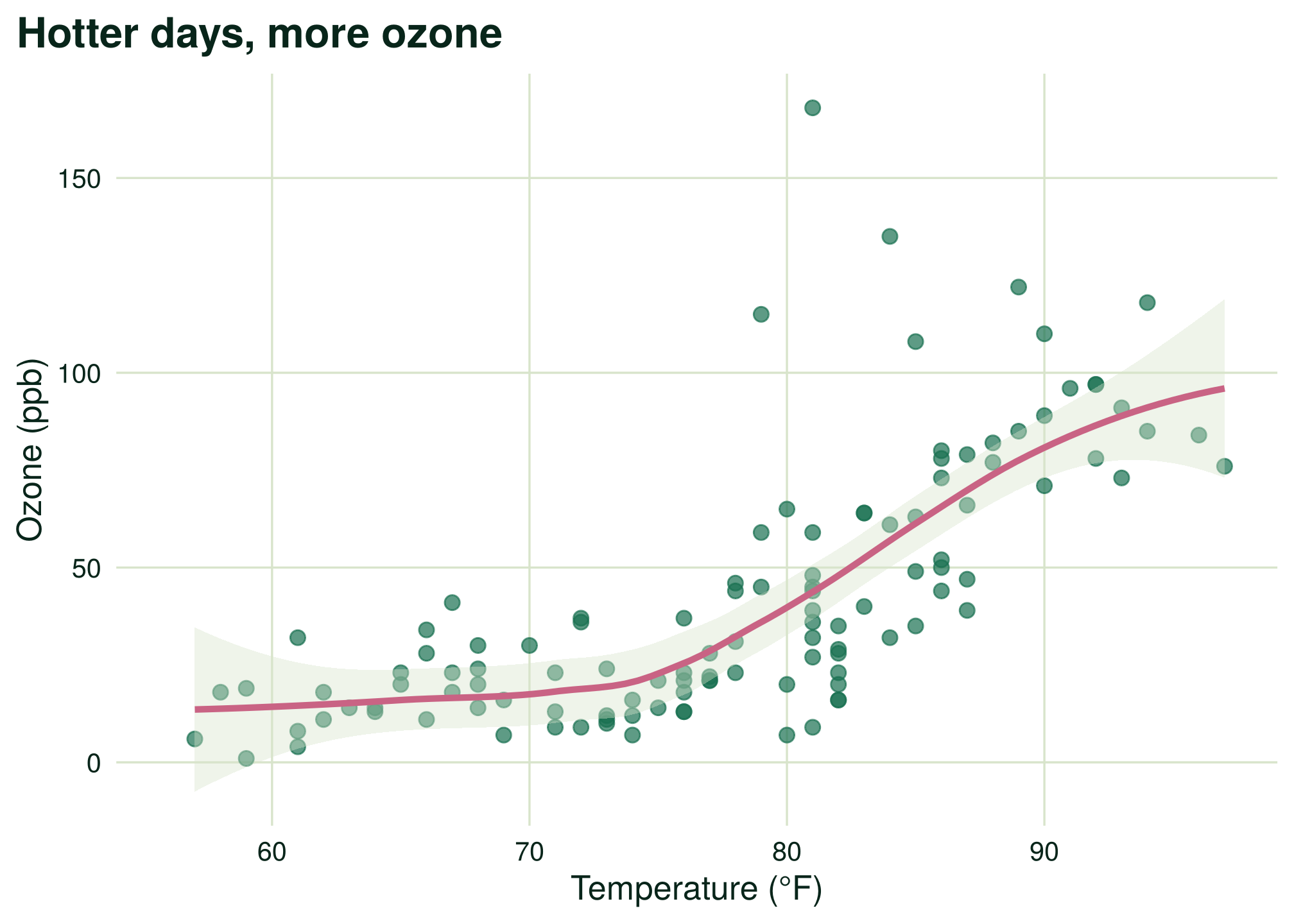
Temperature explains a lot of it

ggplot(aq, aes(Temp, Ozone)) +
  geom_point(colour = fn_cols[["forest_500"]], alpha = 0.7, size = 2.4) +
  geom_smooth(colour = fn_cols[["pink"]], fill = fn_cols[["sage_200"]], linewidth = 1.2) +
  labs(title = "Hotter days, more ozone", x = "Temperature (°F)", y = "Ozone (ppb)")

Figure 2: Ozone against temperature with a loess smoother.

Note

About a quarter of the ozone readings are missing. ggplot2 drops them quietly, which is fine for a sketch but worth handling properly in real work.