flowchart LR
  A[Define an angle<br/>for every point] --> B[Scatter particles]
  B --> C[Look up the angle<br/>under each particle]
  C --> D[Step a little way<br/>in that direction]
  D --> C
  D --> E[Draw the paths]
Flow fields from scratch in Python
Particles drifting through a grid of angles: the gateway drug of generative art.
Art
Python
generative
How flow fields work, built up step by step in NumPy and matplotlib: the field, one particle, thousands of particles, smoother noise and a few variations.
If you’ve seen generative art that looks like hair, smoke, wind or wood grain, there’s a good chance it was a flow field. The idea is tiny: cover the canvas with arrows, drop some particles on it, and let each particle follow the arrow underneath it. The arrows decide the shape, the particles reveal it.
This post builds one from scratch in NumPy and matplotlib. No creative-coding framework, nothing to install beyond what you already have for data work.
The recipe
1. The field
A flow field is a function that takes a position (x, y) and returns an angle. Any function will do. Here’s one made from a couple of sine waves:
def angle(x, y):
    return 3.2 * np.sin(2.4 * x) * np.cos(3.1 * y) + 1.4 * np.sin(5 * y)
Drawing the angle as an arrow at each point of a coarse grid shows the “wind” the particles will feel:
xs, ys = np.meshgrid(np.linspace(0, 1, 40), np.linspace(0, 0.62, 25))
a = angle(xs, ys)

fig, ax = plt.subplots(figsize=(9, 5.6), facecolor="white")
ax.quiver(xs, ys, np.cos(a), np.sin(a), a, cmap="viridis", pivot="mid",
          scale=55, width=0.0025, headwidth=3.5)
ax.set_aspect("equal"); ax.set_axis_off()
plt.show()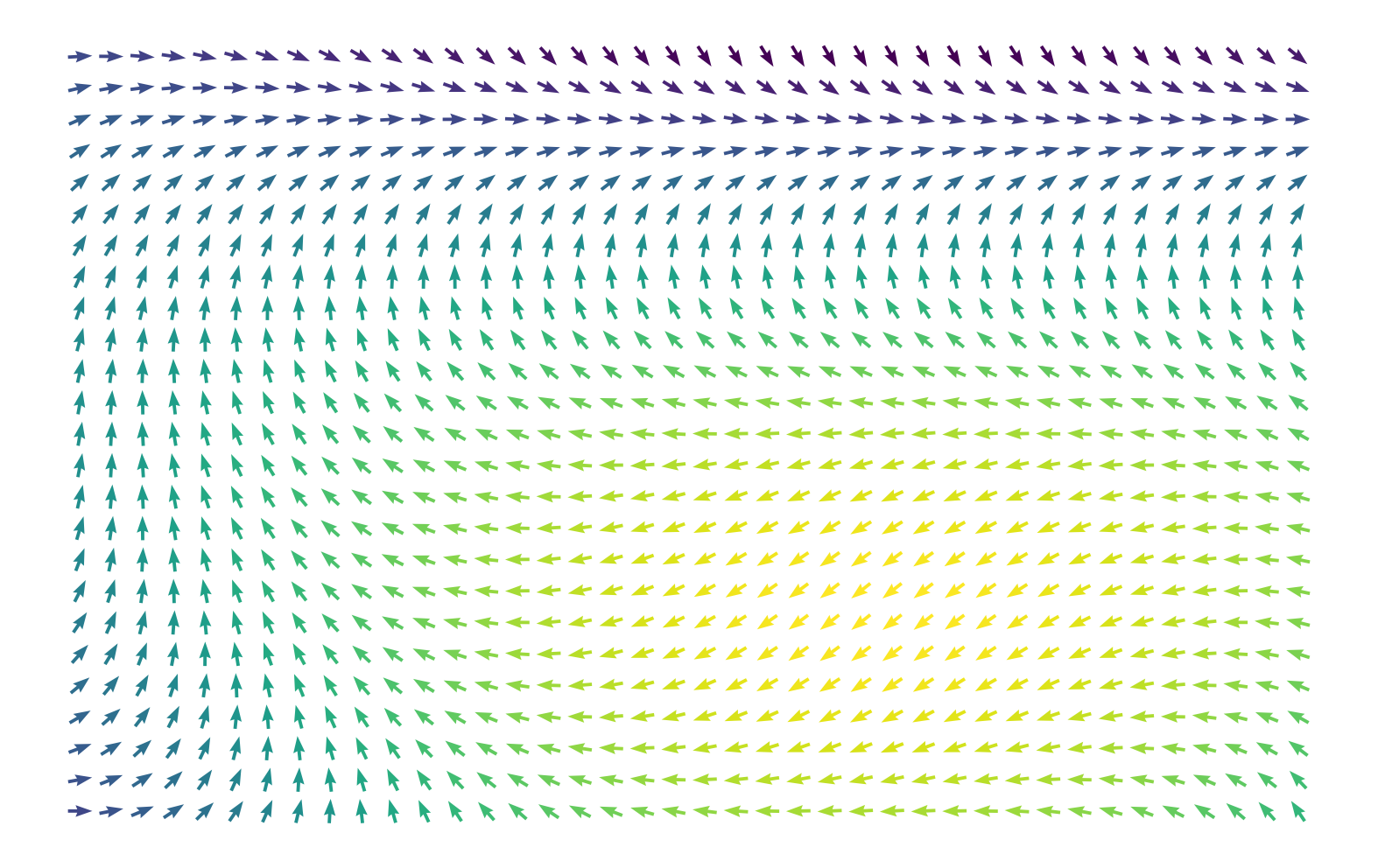
You can already see the structure: swirls, ridges and calm channels. Everything that follows is just a nicer way of looking at this picture.
2. One particle
A particle starts somewhere, reads the angle under it, takes a small step in that direction and repeats. That’s Euler integration, the simplest possible way to follow a field.
def trace(x, y, steps=200, step_size=0.004):
    path = [(x, y)]
    for _ in range(steps):
        a = angle(x, y)
        x, y = x + step_size * np.cos(a), y + step_size * np.sin(a)
        path.append((x, y))
    return np.array(path)
fig, ax = plt.subplots(figsize=(9, 5.6), facecolor="white")
ax.quiver(xs, ys, np.cos(a), np.sin(a), color="#d8e4cb", pivot="mid",
scale=55, width=0.0025, headwidth=3.5)
for (x0, y0), c in zip([(.1, .1), (.3, .5), (.55, .2), (.75, .45), (.9, .1)],
["#197050", "#2f9b99", "#c96384", "#e0a526", "#3ab533"]):
p = trace(x0, y0)
ax.plot(p[:, 0], p[:, 1], lw=3, color=c, solid_capstyle="round")
ax.plot(x0, y0, "o", ms=9, color=c, mec=FOREST, mew=1.5)
ax.set_xlim(0, 1); ax.set_ylim(0, .62); ax.set_aspect("equal"); ax.set_axis_off()
plt.show()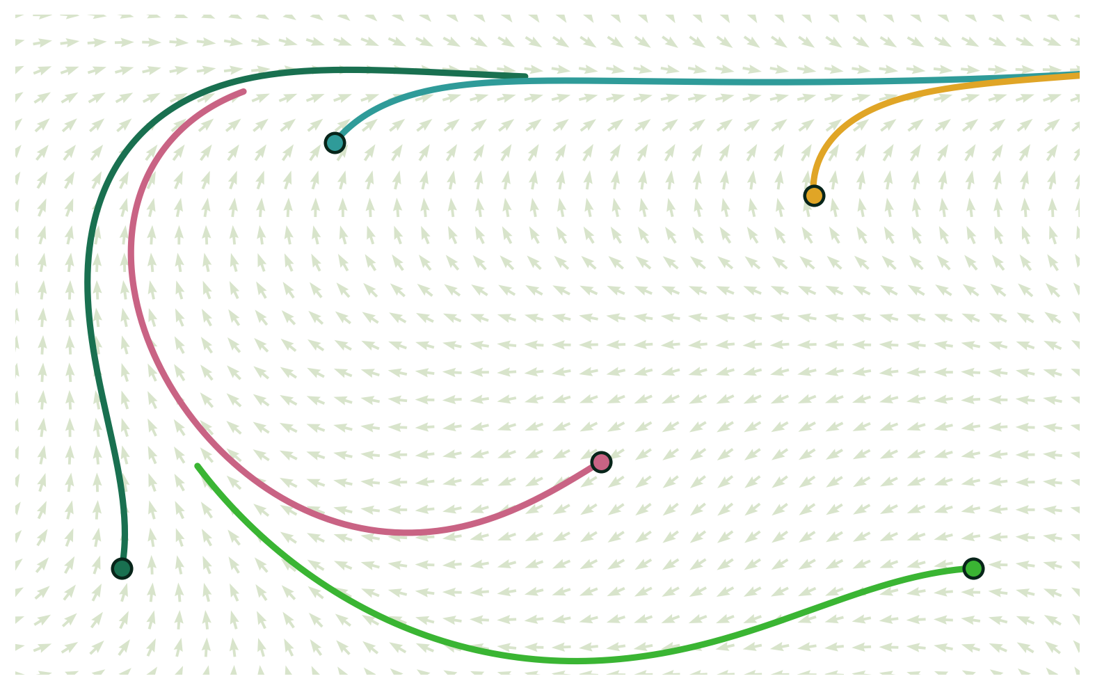
3. Thousands of particles
Tracing particles one at a time in a Python loop gets slow. NumPy lets us move all of them at once: keep their positions in two arrays and update every particle in each step. LineCollection then draws thousands of paths in one go.
def flow(angle_fn, n=2000, steps=140, step_size=0.0035, seed=7, w=1.0, h=0.62, starts=None):
    """Return an (n, steps+1, 2) array of particle paths."""
    rng = np.random.default_rng(seed)
    if starts is None:
        x, y = rng.uniform(0, w, n), rng.uniform(0, h, n)
    else:
        x, y = starts
    paths = np.empty((len(x), steps + 1, 2))
    paths[:, 0] = np.column_stack([x, y])
    for i in range(1, steps + 1):
        a = angle_fn(x, y)
        x, y = x + step_size * np.cos(a), y + step_size * np.sin(a)
        paths[:, i] = np.column_stack([x, y])
    return paths

def draw(paths, colours, bg=FOREST, lw=0.7, alpha=0.6, size=(10, 6.2), ax=None, w=1.0, h=0.62):
    if ax is None:
        fig, ax = plt.subplots(figsize=size, facecolor=bg)
    ax.set_facecolor(bg)
    cols = [colours[i % len(colours)] for i in range(len(paths))]
    ax.add_collection(LineCollection(paths, colors=cols, linewidths=lw, alpha=alpha,
                                     capstyle="round"))
    ax.set_xlim(0, w); ax.set_ylim(0, h); ax.set_aspect("equal")
    ax.set_xticks([]); ax.set_yticks([])          # hide axes but keep the background
    for spine in ax.spines.values():
        spine.set_visible(False)
    return ax
draw(flow(angle), DUSK)
plt.show()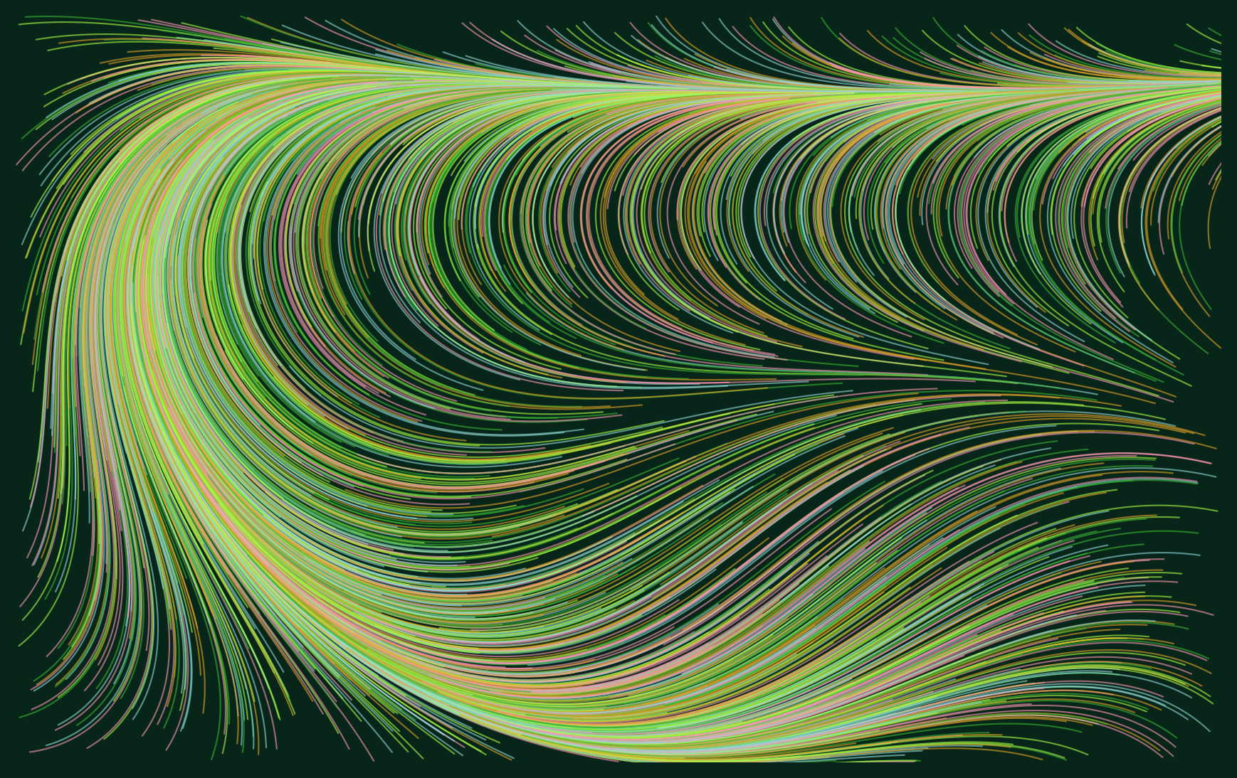
That’s the core technique. The rest of this post is about changing one ingredient at a time.
4. Smoother fields with noise
Sine waves repeat, and you can feel the repetition. Most flow-field art uses noise instead: smooth randomness that wanders without repeating. Perlin noise is the classic choice, but a simple “value noise” does the job in a few lines. It works like this: put random numbers on a coarse grid, blend smoothly between them, then add a few finer layers on top.
def value_noise(seed=1, res=6, octaves=3):
    rng = np.random.default_rng(seed)
    grids = [rng.random((res * 2**o + 2, res * 2**o + 2)) for o in range(octaves)]

    def sample(x, y):
        total, amp, norm = 0.0, 1.0, 0.0
        for o, g in enumerate(grids):
            r = res * 2**o
            gx, gy = np.clip(x, 0, 1) * r, np.clip(y / 0.62, 0, 1) * r
            i, j = gx.astype(int), gy.astype(int)
            fx, fy = gx - i, gy - j
            fx, fy = fx * fx * (3 - 2 * fx), fy * fy * (3 - 2 * fy)   # smoothstep
            top = g[j, i] * (1 - fx) + g[j, i + 1] * fx
            bot = g[j + 1, i] * (1 - fx) + g[j + 1, i + 1] * fx
            total += amp * (top * (1 - fy) + bot * fy)
            norm += amp; amp *= 0.5
        return total / norm
    return sample

noise = value_noise(seed=3)
noise_angle = lambda x, y: noise(x, y) * 4 * np.pi
draw(flow(noise_angle, n=2500, steps=160), GREENS, alpha=0.55)
plt.show()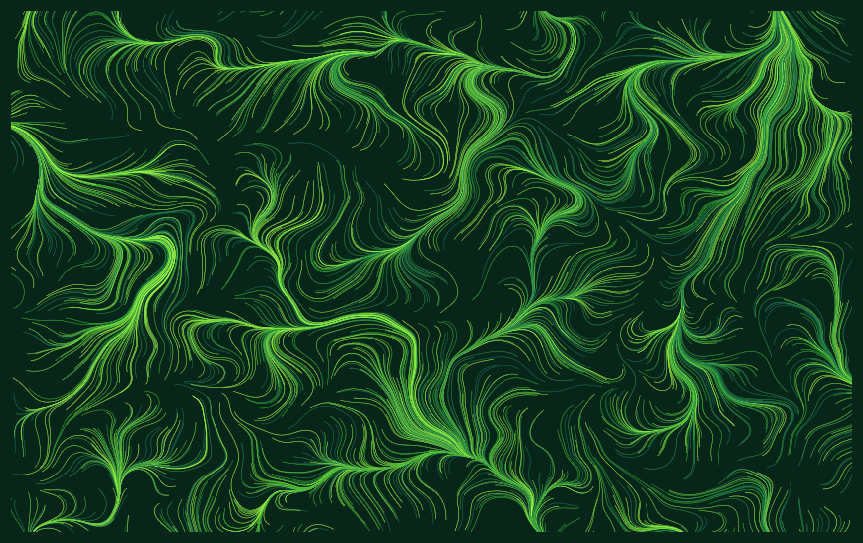
5. Variations
Small changes go a long way. Three to try:
- Where particles start. Seeding them on a circle gives you rings and ribbons.
- How lines are drawn. Thick, short and opaque reads as brush strokes, while thin, long and translucent reads as silk.
- The palette. Dark ground with bright lines, or the reverse.
fig, axes = plt.subplots(1, 3, figsize=(15, 3.4), facecolor="white",
                         gridspec_kw={"wspace": 0.03})

t = np.linspace(0, 2 * np.pi, 900, endpoint=False)
ring = (0.5 + 0.2 * np.cos(t), 0.31 + 0.2 * np.sin(t))
draw(flow(noise_angle, steps=120, starts=ring), DUSK, ax=axes[0], lw=0.8)

draw(flow(noise_angle, n=900, steps=18, step_size=0.006, seed=2), GREENS,
     ax=axes[1], lw=3.2, alpha=0.9)

draw(flow(angle, n=1600, steps=160, seed=4), [FOREST, "#197050", "#2f9b99"],
     bg="#eff6e9", ax=axes[2], lw=0.5, alpha=0.5)
plt.show()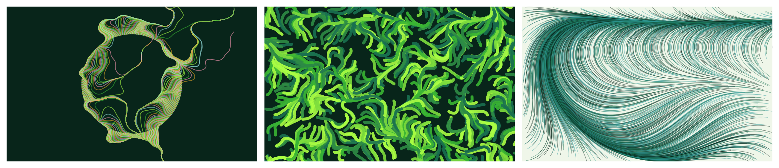
6. A finished piece
Putting it together: noise field, many long paths, the blog’s greens over a dark forest ground, and a scattering of lime “fireflies” where some particles end their paths.
paths = flow(noise_angle, n=4000, steps=180, step_size=0.003, seed=11)
ax = draw(paths, GREENS[1:] + ["#2f9b99"], lw=0.45, alpha=0.5, size=(11, 6.8))
ends = paths[::25, -1]
ax.scatter(ends[:, 0], ends[:, 1], s=6, color="#abff44", alpha=0.9, linewidths=0)
plt.show()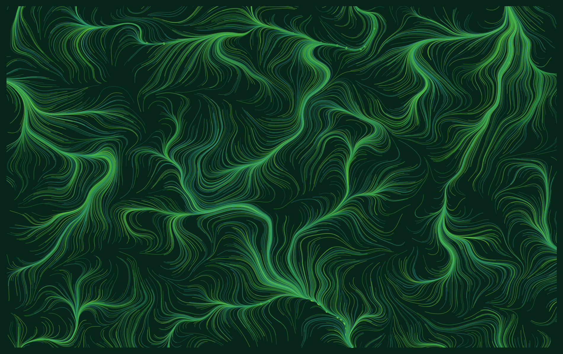
Things to try next
- Stop paths from crossing. Track which grid cells are already used and end a particle when it enters one. This gives the clean, evenly spaced look you see in a lot of plotter art.
- Colour by angle. Map each segment’s direction to a colour instead of picking colours by index.
- Animate it. Increase
stepsframe by frame and save the frames withmatplotlib.animation. - Read the classic essay. Tyler Hobbs’ Flow Fields is the best long read on the technique.
The field decides the shape. The particles only reveal it.